

SAGE: Semi-Automatic Ground Environment Air Defense System
The Semi-Automatic Ground Environment, or SAGE, was the nation's first air defense system and was the impetus for the establishment of Lincoln Laboratory. The sections below describe the history of this seminal, large-scale system-engineering project, and the role that it had in shaping the culture of Lincoln Laboratory as it exists today.
A New Threat
On September 3, 1949, a U.S. Air Force WB-29 aircraft from the 375th Weather Reconnaissance Squadron landed at Eielson Air Force Base, Alaska, with filter paper samples collected east of the Soviet Union's Kamchatka Peninsula. Tests on the samples showed anomalously high levels of airborne radioactive debris — high enough to be explained only by an atomic explosion.

Intelligence sources in the United States reported that scientists in the Soviet Union were pushing hard to develop a nuclear capability, but it appeared that they were having trouble. The consensus was that the Soviets were still about three years away from completing a working atomic bomb. Nevertheless, the United States began routine monitoring to detect atomic explosions in the Soviet Union.
The radioactive filter paper samples were flown to a lab in Berkeley, California, and the test results were reported to the Air Force. Independent tests were conducted by the Los Alamos Scientific Laboratory, by the British Atomic Energy Authority on airborne samples collected north of Scotland, and by the Naval Research Laboratory on rainwater collected in Kodiak, Alaska, and in Washington, D.C. Each of the tests confirmed high levels of radioactivity.
On September 19, Vannevar Bush, then president of the Carnegie Institution, convened a special panel in Washington, D.C. This panel formally concluded that the USSR had exploded its first atomic bomb, code-named Joe-1, on August 29, 1949.

The announcement by President Harry Truman on September 23, 1949, of an atomic explosion by the Soviet Union shocked the nation. Even worse news came out a short time later. Not only did the Soviet Union have the bomb, it had also developed long-range aircraft able to reach the United States via an Arctic route. The United States had no defense against nuclear attack. The Ground Control of Intercept (GCI) radar network developed during World War II had been designed to defend against an attack with conventional weapons, and it had only a limited ability to detect incoming hostile aircraft. A wave of Soviet bombers carrying nuclear weapons would almost certainly succeed in evading detection by these radars.

A sense of fear and helplessness began to pervade the United States. Civil defense groups built air-raid shelters, and parents trained their children for the possibility of a nuclear war. Today, these perceptions and actions might seem unrealistic and excessive, but in 1949 these fears were very real.
The United States had grown accustomed to having a monopoly on nuclear weapons. Americans had felt invulnerable, and efforts to maintain military installations had been reduced to minimal levels. The Soviet Union's atomic bomb ended this period of complacency, and the USSR became the Red Menace. Stories about Joseph Stalin's purges and labor camps, though incomplete, further enhanced the feeling of dread. That Stalin might use nuclear weapons seemed entirely plausible.
These perceptions compelled the Department of Defense (DoD) to reevaluate the nation's defenses against nuclear attack. As a part of the process, the DoD assigned the U.S. Air Force the task of improving the nation's air defense system. The Air Force, in turn, asked the Massachusetts Institute of Technology for assistance — and this led to the formation of MIT Lincoln Laboratory.
Lincoln Laboratory Origins
The story of Lincoln Laboratory begins with George Valley. An associate professor in the MIT Physics Department, Valley was well known for his concern over nuclear weapons. In 1949, after learning of the Soviet atomic bomb, Valley became worried about the quality of U.S. air defenses. Conversations with other professors led him to conclude that the United States had virtually no protection against nuclear attack.
In his concern over the possibility of nuclear attack, George Valley was like many Americans. But in his desire to address the problem, he was unique. Valley decided to make the task of securing U.S. air defenses his personal responsibility.
Valley was in an excellent position to evaluate U.S. air defenses. As a member of the Air Force Scientific Advisory Board (SAB), he was able to arrange a visit to a radar station operated by the Air Force Continental Air Command. What he saw appalled him. The equipment had been brought back from World War II and was inappropriate for detecting long-range aircraft. Moreover, the operators had received only minimal instruction in the problems of air defense. He was particularly struck by the site's use of high-frequency (HF) radios; the quality of HF communications is dependent on the state of the ionosphere, which can vary over time and would be severely disturbed in the event of a nuclear explosion.
Following his visit to the radar station, Valley collected more information on U.S. air defenses, none of it reassuring, and then called Theodor von Karman, chairman of the SAB. Von Karman asked Valley to put his concerns in writing, which he did in a letter dated November 8, 1949.
Von Karman relayed Valley's concerns to General Hoyt Vandenberg, the Air Force chief of staff. Vandenberg instructed his vice chief of staff, General Muir Fairchild, to take immediate action. By December 15, Fairchild had organized a committee of eight scientists, with Valley as the chair, to analyze the air defense system and to propose improvements. On January 20, 1950, the committee, officially named the Air Defense Systems Engineering Committee (ADSEC) but informally known as the Valley Committee, began to meet weekly.
The Valley Committee
The members of the Committee agreed to begin their study with a set of basic assumptions about hostile aircraft and U.S. air defenses. They agreed that a Soviet bomber would most likely fly over the north polar region at high altitude and then descend as it approached its target. While the aircraft flew at high altitude, it would be able to detect ground radar before the radar could detect the aircraft. The bomber could then descend to a low altitude, where it could fly under the beam of the radar and be virtually undetectable. The committee determined that, to attack a city in the United States, a Soviet bomber would need to fly at low altitude for only about 10 percent of its journey. Therefore, the range penalty for low-altitude flight would be small. If aerial refueling were performed near the Arctic Circle, the entire United States could be vulnerable to a Soviet attack. Spaced as they were, the then-existing GCI radars gave virtually no protection. A low-flying aircraft could find a clear path to almost every city in the United States.
The Committee determined that the weakest link in the nation's air defenses was the radars that were supposed to detect low-flying aircraft. Each radar's range was limited by its horizon. By flying at low altitude, aircraft could hide from the widely spaced GCI radars. Since air-based or space-based surveillance was not an option in 1950, the only solution was to install ground-based radar systems close together.
In 1950, this solution was ambitious. But fortunately for the future Lincoln Laboratory, the Committee continued to evaluate the problem and reduced it to two major issues. First, in order to interpret the signals from a large number of radars, there had to be a way to transmit the radar data to a central computer at which the data could be aggregated. Second, since the objective was to detect and intercept the hostile aircraft, the computer had to analyze the data in real time.
When Valley called several computer manufacturers to inquire about the possibility of using one of their systems to test his ideas, he was dismissed as a crackpot. Real-time operation was simply inconceivable in 1950. However, the answers to the problems of data transmission and of real-time operation were waiting to be addressed nearby. At the Air Force's Cambridge Research Laboratory, John Harrington had developed an early form of modem known as the digital radar relay, which was capable of converting analog radar signals into digital code that could be transmitted over telephone lines. Also, at the Servomechanisms Laboratory on the MIT campus, Jay Forrester was heading up a group that was developing the world's first real-time computer.
Valley needed a computer fast enough to handle real-time data analysis. As he began his search, Valley ran into Professor Jerome Wiesner, then associate director of the Research Laboratory of Electronics, and learned that the computer he required was already on the MIT campus. It was in the Servomechanisms Laboratory, and it was about to be abandoned by its sponsor.
During World War II, the emphasis in the Servomechanisms Laboratory had been on developing gun-positioning instruments. After the end of the war, the laboratory had begun a program to demonstrate a flight simulator for the Office of Naval Research. Plans had called for this device to simulate virtually every aircraft then in existence. Because this would require a powerful computer, the Servomechanisms Laboratory had begun to develop its own computer, code-named Whirlwind.
From his talk with Forrester, Valley was convinced that Whirlwind was suited to the ADSEC project. From then on, Forrester was a regular participant in ADSEC. Whirlwind was in a relatively early stage of its construction, with only 5 words of random-access memory and 27 words of programmable read-only memory. Yet its high speed and 16-bit word length made it adequate for ADSEC to test the feasibility of the concept that radar data could be transmitted to a computer via the digital radar relay, and that the computer could respond to the information in real time and direct an interception.

Forrester promptly began preparing to receive and process digitized radar signals. The feasibility demonstration of the radar/digital-data concept took place at Hanscom Field in September 1950. The radar, which was an original experimental model of a microwave early-warning unit built by the wartime MIT Radiation Laboratory, closely resembled the radars used in the D-Day invasion of Normandy. While military observers watched closely, an aircraft flew past the radar, the digital radar relay transmitted the signal from the radar to Whirlwind via a telephone line, and the result appeared on the computer's monitor. The demonstration was a complete success and proved the feasibility of ADSEC's air defense concept.
The demonstration at Hanscom Field signaled the end of the first phase of ADSEC's work. The committee's focus shifted from evaluation to implementation; a laboratory dedicated to air defense problems began to be discussed.
On November 20, 1950, Louis Ridenour, chief scientist of the Air Force, wrote in a memo to Major General Gordon Saville, deputy chief of staff for development in the Air Force, "It is now apparent that the experimental work necessary to develop, test, and evaluate the systems proposals made by ADSEC will require a substantial amount of laboratory and field effort."
Ridenour's memo was the first document to propose a laboratory dedicated to air defense research. He estimated that such a laboratory would require a staff of about 100 and a budget of about $2 million per year. (During the 1950s, Lincoln Laboratory actually would have a staff of about 1800 and an annual budget in excess of $20 million.)
A few weeks later, on December 15, Valley joined Ridenour for lunch at the Pentagon. Ridenour persuaded Valley that they should ask MIT to set up the electronics laboratory that could develop ADSEC's air defense ideas. Valley later recalled that he wrote a letter in about an hour and that Ridenour recast it in "appropriate general officer's diction." By four o'clock, the letter had been signed by General Vandenberg and was on its way to James Killian, Jr., president of MIT.
The Vandenberg letter to Killian contained the following text:
The Air Force feels it is now time to implement the work of the part-time ADSEC group by setting up a laboratory which will devote itself intensively to air defense problems…
The Massachusetts Institute of Technology is almost uniquely qualified to serve as contractor to the Air Force for the establishment of the proposed laboratory. Its experience in managing the Radiation Laboratory of World War II, the participation in the work of ADSEC by Professor Valley and other members of the MIT staff, its proximity to AFCRL [Air Force Cambridge Research Lab] and its demonstrated competence in this sort of activity have convinced us that we should be fortunate to secure the services of MIT in the present connection.
The air defense problem which faces the Air Force is of great importance to the people of this country. The problem is technically complicated and difficult. The Air Force must urgently increase its research and development effort in this area and in this we ask your help. I sincerely hope that you will be able to give the matter serious consideration.
MIT Establishes the New Laboratory
Project Charles
MIT President James Killian had serious reservations about MIT starting up a new laboratory because MIT had "devoted itself so intensively to the conduct of the Radiation Laboratory and other large war projects."

Louis Ridenour, chief scientist of the U.S. Air Force, provided President Killian with a reason for setting up a laboratory that, although unrelated to national defense, was particularly persuasive. Ridenour suggested that a laboratory to address air defense problems would serve as a stimulus for the nation's small electronics industry. He predicted that the state that became the home of the new laboratory would emerge as a center for the electronics industry. Ridenour's words were prophetic, as evidenced by the growth of the electronics and computer industry along Route 128, the circumferential highway around Boston.
Because Killian was not eager for MIT to become involved in air defense, he asked the Air Force if MIT could first conduct a study to evaluate the need for a new laboratory and to determine its scope. Killian's proposal was approved, and a study named Project Charles (for the river that flows past MIT) was carried out between February and August 1951.
Project Charles was conducted by a group of 28 scientists, 11 of whom were associated with MIT. The director was F. Wheeler Loomis, the University of Illinois professor who subsequently became Lincoln Laboratory's first director. Albert Hill and Carl Overhage, also members of the study, became the Laboratory's second and fourth directors, respectively. Most of the other members of Project Charles also went on to join the Laboratory.
The Final Report of Project Charles stated that the United States needed an improved air defense system and that Valley had developed the correct plan: "We endorse the concept of a centralized system as proposed by the Air Defense Systems Engineering Committee, and we agree that the central coordinating apparatus of this system should be a high-speed electronic digital computer."
Project Charles came out unequivocally in support of the formation of a laboratory dedicated to air defense problems:
Experimental work on certain of these problems is planned in a laboratory to be operated by the Massachusetts Institute of Technology jointly for the Army, the Navy, and the Air Force, to be known as PROJECT LINCOLN.1
This statement was the approval by a technically trained panel that President Killian had wanted. The decision to found the new laboratory, with the unusual support of all three services, became final.
1 Problems of Air Defense: Final Report of Project Charles, Vol. I. Cambridge, Mass.: MIT, 1951, p. x.
Project Lincoln
The Charter for the Operation of Project Lincoln stated that the Air Force was to build a laboratory where the Massachusetts towns of Bedford, Lexington, and Lincoln meet. Why the name Lincoln? There had already been a Project Bedford (on antisubmarine warfare) and a Project Lexington (on nuclear propulsion of aircraft), so Major General Putt, who was in charge of drafting the Charter, decided to name the project for the town of Lincoln.
F. Wheeler Loomis took over as director of Project Lincoln. He had a small staff, unsure funding, and a promise to construct a laboratory. Moreover, he faced an immense challenge — to design a reliable air defense system for the continent of North America. Before Loomis could begin to hire the staff for Project Lincoln, he had to set up a structure for the organization. For this, he drew upon a model originated by the Radiation Laboratory in 1942. The organizational structure he followed consisted of a director's office, a steering committee, and a staff divided into divisions and groups. Each division was in charge of developing a system, and each group designed a component of that system. The concept of divisions and groups proved effective and efficient. Its simplicity enabled Project Lincoln to operate with far fewer managers and with far less internal politics than many other organizations. In fact, the structure worked so well that it has remained in use in Lincoln Laboratory to this day.
Project Lincoln was divided into five technical divisions: aircraft control and warning, communications and components, weapons, special systems, and digital computers. It also had two service divisions: business administration and technical services. The divisions were divided into one to six groups. Each division examined one aspect of the continental air defense problem; each group looked at one element of its division's task.
By September 1951, Project Lincoln had more than 300 employees. Within a year, it employed 1,300. One year later, Lincoln Laboratory had grown to 1,800 personnel, a level that would remain fixed for several years.
With staff coming on board and the funding secure, Loomis now turned his attention to the construction of buildings. The space on the MIT campus was already inadequate, and hundreds of employees were joining the project. The sole site available on campus for classified work was Building 22.
Unclassified research was carried out in Building 20, and administrative offices of Project Lincoln were located in the Sloan Building at MIT. Temporary housing for the motor pool, the electronics shops, and the publications office was found in a two-story commercial building on Vassar Street. Although the MIT Digital Computer Laboratory (originally part of the Servomechanisms Laboratory) became part of Project Lincoln, work on Whirlwind continued to be carried out in the Barta Building on Massachusetts Avenue and in the Whittemore Building on Albany Street.
Space was not the only issue. President Killian believed that MIT should not be carrying out classified research on the Cambridge campus. He thought that MIT had an obligation to disseminate its research results throughout the academic community and that classified research was inherently incompatible with this obligation. Therefore, Killian wanted MIT to maintain its integrity by conducting Project Lincoln off campus. The Bedford-Lincoln-Lexington area mentioned in the Charter for the Operation of Project Lincoln had space for new construction, and it was a comfortable distance from Cambridge.
This site was the Laurence G. Hanscom Field, now Hanscom Air Force Base and still the home of Lincoln Laboratory. Hanscom Field became a Commonwealth of Massachusetts facility in May 1941, when the state legislature acquired 509 acres for the construction of an airport. It was located in part in each of the towns of Concord, Lincoln, Lexington, and Bedford, on a flat area between the Concord and Shawsheen rivers. The official groundbreaking ceremony for the airfield, then known simply as the Boston Auxiliary Airport at Bedford, was held on June 26, 1941.
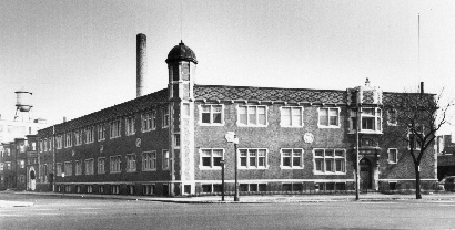
Lincoln Laboratory
Groundbreaking for Project Lincoln began in 1951 at the foot of Katahdin Hill in Lexington. The site lay directly below 47 acres of farmland that had been acquired by MIT in 1948 as a site for cosmic-ray research. Twenty-six acres were transferred to the Army, and the remaining 21 acres were assigned to Project Lincoln.
The new buildings were laid out in an open-wing configuration, with alternate wings along a central axis. The plans called for four wings (Buildings A, B, C, and D) plus a concrete block utility structure (Building E).
The Boston firm of Cram and Ferguson was chosen as the architect. Although the firm was among the oldest and largest of its kind in the United States, it was not generally associated with laboratory construction. In fact, the firm was better known for Gothic and art deco architecture, such as the Cathedral of St. John the Divine in New York City and the 1948 John Hancock Building in Boston.
Cram and Ferguson came up with a modular design for the buildings, with each staff member allotted 9 × 9 square feet. The main corridor of each building was 400 feet long, which yielded 44 modules along each side. Supporting columns were spaced 18 feet apart, and movable partitions were used for the internal walls.

Buildings were 60 feet wide, with 15 feet wide corridors. Because laboratories required more space than offices, modules were 18 feet deep on one side of the corridor and 27 feet deep on the other. Buildings B and C each had four stories, three above and one below ground level. Buildings A and D had three stories, and the lowest levels were only partially below ground. Building E had a single story and a small basement. It held the receiving room, stockroom, storage area, shops, and garage.
Building B was completed barely two years after the first meeting of ADSEC and less than a year after the Project Charles Final Report. The scientists and engineers working on Project Lincoln were talented indeed, as are so many working at Lincoln Laboratory today. But the MIT Radiation Laboratory had instituted procedures that were remarkably free of red tape, and this was its legacy to Project Lincoln.

Fear of nuclear holocaust pervaded the thinking of Americans in the 1950s, and the government of the United States was committed to protecting the country against this threat. Because Project Lincoln's mission was vital to the security of the nation, red tape was eliminated at all stages.
The Air Force had put its resources at the disposal of Project Lincoln. Now, the staff had only one more problem to solve: they had to deliver a reliable air defense system for North America.
The SAGE Air Defense System
The scope of the SAGE Air Defense System, as it evolved from its inception in 1951 to its full deployment in 1963, was enormous. The cost of the project, both in funding and the number of military, civilian, and contractor personnel involved, exceeded that of the Manhattan Project. The project name evolved over time from Project Lincoln, its original 1951 designator, to the Lincoln Transition System, and finally settled out as the Semi-Automatic Ground Environment, or SAGE.
The basic SAGE architecture was cleanly summarized in the preface to a seminal 1953 technical memo written by George Valley and Jay Forrester: Lincoln Laboratory Technical Memorandum No. 20, A Proposal for Air Defense System Evolution: The Transition Phase.
Briefly, the… system will consist of: (1) a net of radars and other data sources and (2) digital computers that (a) receive the radar and other information to detect and tract aircraft, (b) process the track data to form a complete air situation, and (c) guide weapons to destroy enemy aircraft.
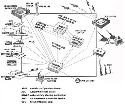
The concept of operations for SAGE was fairly simple and was similar to that of modern automated air defense systems. However, it was pioneering at the time. A large network of radars would automatically detect a hostile bomber formation as it approached the U.S. mainland from any direction. The radar detections would be transmitted over telephone lines to the nearest SAGE direction center, where they would be processed by an AN/FSQ-7 computer. The direction center would then send out notification and continuous targeting information to the air bases best situated to carry out interception of the approaching bombers, as well as to a set of surface-to-air missile batteries. The direction center would also send data to and receive data from adjoining centers, and send situational awareness information to the command centers. As the fighters from the air bases scrambled and became airborne, the direction center would continue to process track data from multiple radars and would transmit updated target positions in order to vector the intercepting aircraft to their targets. After the fighter aircraft intercepted the approaching bombers, they would send raid assessment information back to the direction center to determine whether additional aircraft or missile intercepts were necessary.

- Early warning radar detects approaching aircraft
- Radar reports automatically transmitted to direction center (DC) via phone lines
- DC processes data
- Air bases, HQs, and missile batteries notified
- Data relayed between DC and adjoining centers
- DC assigns interceptor aircraft and vectors interceptors to targets
- Interceptors rendezvous with and intercept targets
- DC informs HQ of results; missile batteries provide second line of defense if needed
The SAGE system, by the time of its full deployment, consisted of 100s of radars, 24 direction centers, and 3 combat centers spread throughout the U.S. The direction centers were connected to 100s of airfields and surface-to-air missile sites, providing a multilayered engagement capability. Each direction center housed a dual-redundant AN/FSQ-7 computer, evolved from MIT's experimental Whirlwind computer of the 1950s. These computers hosted programs that consisted of over 500,000 lines of code and executed over 25,000 instructions — by far the largest computer programs ever written at that time. The direction centers automatically processed data from multiple remote radars, provided control information to intercepting aircraft and surface-to-air missile sites, and provided command and control and situational awareness displays to over 100 operator stations at each center. It was far and away the most grandiose systems engineering effort — and the largest electronic system-of-systems "ever contemplated."

Although the basic concept for SAGE was simple, the technological challenges were immense. One of the greatest immediate challenges was the need to develop a digital computer that could receive vast quantities of data from multiple radars and perform the real-time processing to produce targeting information for intercepting aircraft and missiles. Fortunately, and serendipitously, the initial concept development for such a computer was taking place on the MIT campus in the Servomechanisms Laboratory, under the direction of Jay Forrester. This effort, with its maturation under SAGE, laid the foundation for a revolution in digital computing, which subsequently had a profound impact on the modern world.
Early Digital Computing
By 1952, the basic concept for the air defense project was approaching a degree of maturity. A radar network had been assembled, and Lincoln Laboratory was ready to begin testing. MIT’s Whirlwind computer showed promise for providing the real-time computational capability needed for SAGE. However, the reliability of the computer still posed a significant problem. Before plans for a nationwide air defense system could be taken seriously, the computer would have to become much more reliable.
Magnetic-Core Memory
One of the most significant limitations of computers at the time was the storage tubes that were used for internal memory. These tubes were large and slow, and worst of all, they were unreliable. One of the greatest breakthroughs in the development of Whirlwind was the invention of magnetic-core memory. That invention was the key development leading to the widespread adoption of computers for industrial applications because, unlike computers with storage-tube memories, computers with magnetic-core memories were reliable.
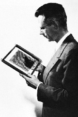
In 1947, while working on Whirlwind in the MIT Servomechanisms Laboratory, Jay Forrester began to think about developing a new type of memory. He conceived of a new way of configuring memory units — in a three-dimensional structure. Although Forrester initially thought of using glow-discharge tubes, preliminary tests indicated that these tubes were too unreliable. Lacking a good way to implement a three-dimensional memory, Forrester dropped work on his concept for a couple of years. Then, in the spring of 1949, he saw an advertisement from the Arnold Engineering Company for a reversibly magnetizable material called Deltamax. Forrester immediately recognized that this was the material he needed for the three-dimensional memory structure.
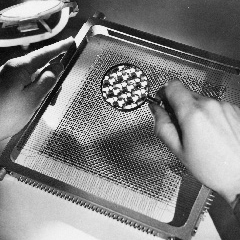
Forrester directed one of his students, William Papian, to study combinations of small toroidal-shaped cores made of ferromagnetic materials possessing suitable hysteresis loop characteristics. Papian's master's thesis, A Coincident-Current Magnetic Memory Unit, completed in August 1950, described the concept of magnetic-core memories and showed how the cores could be combined in planar arrays, which could in turn be connected into three-dimensional assemblies. Papian fabricated the first magnetic-core memory, a 2 × 2 array, in October 1950. The early results were encouraging, and by the end of 1951 a 16 × 16 array of metallic cores was completed.

The organization and direction of Project Whirlwind now went through a major change. The task of developing a flight simulator was abandoned, and the focus of the program shifted to air defense. In September 1951, all members of the Servomechanisms Laboratory who were working on Whirlwind were assigned to a new laboratory — the MIT Digital Computer Laboratory, headed by Jay Forrester. Six months later, the Digital Computer Laboratory was absorbed by Lincoln Laboratory as the Digital Computer Division. Lincoln Laboratory took over the development of magnetic-core memories.
Operation of the early metallic magnetic-core memories was still unsatisfactory — switching times were 30 µsec or longer. Therefore, in cooperation with the Solid State and Transistor Group, Forrester began an investigation of ferrites. These nonconducting magnetic materials had weaker output signals than did the metallic cores, but their switching times were at least ten times faster. In May 1952, a 16 × 16 array of ferrite cores was operated as a memory, with an adequate signal and a switching time of less than a microsecond. So promising was the performance of the new array that the Digital Computer Division began construction of a 32 × 32 × 6 memory, the first three-dimensional memory.
Whirlwind was by this time in considerable demand, so a new machine called the Memory Test Computer was built to evaluate the 16,384-bit core memory. When the Memory Test Computer went into operation in May 1953, the magnetic-core memory, in sharp contrast to the electrostatic-storage-tube memory in Whirlwind, was highly reliable. Forrester promptly removed the core memory from the Memory Test Computer and installed it in Whirlwind.
The first bank of core storage was wired into Whirlwind on August 8, 1953. A month later, a second bank went in. A different memory was subsequently installed in the Memory Test Computer, enabling that machine to be used in other applications.
The improvement in Whirlwind's performance was dramatic. Operating speed doubled; the input data rate quadrupled. Maintenance time on the memory dropped from four hours per day to two hours per week, and the mean time between memory failures jumped from two hours to two weeks.
The invention of core memory was a watershed in the development of commercial computers. The technology was quickly adopted by International Business Machines (IBM), and the first nonmilitary system to use magnetic-core memories, the IBM 704, went on the market in 1955. Magnetic cores were used in virtually all computers until 1974, when they were superseded by semiconductor integrated-circuit memories.
Impact of SAGE on Computing
Computers were in their infancy when George Valley first approached Jay Forrester to discuss developing an air defense network, and the industrial base needed to develop the required computing capability simply did not exist. Therefore, in addition to prototyping and testing the first real-time digital computers, the Project Lincoln staff had to cultivate the industrial infrastructure needed to bring a nation-wide air defense system into being. The result was that the SAGE program became a driving force behind the formation of the American computer and electronics industry in the 1950s.
The modular computer architecture, first developed by Ken Olsen as a staff member at Lincoln Laboratory, became a key part of the programmed data processor (PDP) minicomputer which Olson popularized through the company that he founded, the Digital Equipment Corporation. In addition, the contract to build the AN/FSQ-7 played a sizable role in the metamorphosis of IBM from a business machine vendor to the world's largest computer manufacturer.
The breakthroughs that came about through the course of the SAGE program initiated, to a large extent, the digital computing revolution that has had such a significant impact on today's world.
The AN/FSQ-7 Computer
The Whirlwind project at MIT's Digital Computer Laboratory had demonstrated real-time control, the key ingredient for the Project Lincoln air defense concept. Whirlwind also provided an experimental test bed for the system design. By the spring of 1952, Whirlwind was working well enough to be used as part of the early air defense prototyping activities. The focus of the program within the Digital Computer Division shifted, therefore, to development of a production computer, Whirlwind II.
Whirlwind I was more of a breadboard than a prototype of a computer that could be used in the air defense system. The Whirlwind II group dealt with a wide range of design questions, including whether transistors were ready for large-scale employment (they were not) and whether the magnetic-core memories were ready for exploitation as a system component (they were). The most important goal for Whirlwind II was that there should be no more than a few hours of down time per year.
The AN/FSQ-7 computer was designed by joint Lincoln Laboratory and IBM committees that managed to merge the best elements of their members' diverse backgrounds to produce a result that advanced the state of the art in many directions.
To turn the ideas and inventions developed in the Whirlwind program into a reproducible, maintainable operating device required the participation of an industrial contractor. A team, led by Jay Forrester, was set up to evaluate potential contractors. This team was responsible for finding the most appropriate computer designer and manufacturer to translate the progress made in Project Lincoln into a design for an operational air defense system. The team surveyed the possible engineering and manufacturing candidates and chose three for further evaluation: IBM, Remington Rand, and Raytheon. They visited each company, reviewed its capabilities, and graded each on the basis of personnel, facilities, and experience.
IBM received the highest score and was issued a six-month subcontract in October 1952. Over the next few months, the IBM group visited Lincoln Laboratory frequently to study the system being developed, to become acquainted with the overall design strategy, and to learn the specifics of the central processor design.
In January 1953, system design for Whirlwind II began in earnest. The computer was designed by joint Lincoln Laboratory and IBM committees that managed to merge the best elements of their members' diverse backgrounds to produce a result that advanced the state of the art in many directions.
The schedule was tight. Lincoln Laboratory set a target date of January 1, 1955, to complete the prototype computer and its associated equipment. Installation, testing, and integration of the equipment in the air defense system were scheduled to be started on July 1, 1954. The nine months preceding this, October 1, 1953, to July 1, 1954, would be needed for procurement of materials and construction. The schedule left about nine months for engineering tasks in connection with the preparation of specifications, block-diagram work, development of basic circuit units, special equipment design, and everything else necessary before construction could begin.
In April 1953, IBM received a prime contract to design the computer. A short time later, the name Whirlwind II was dropped in favor of Air Force nomenclature, and the computer was designated AN/FSQ-7. In September, IBM received a contract to build two single-computer prototype systems, AN/FSQ-7(XD-l) and AN/FSQ-7(XD-2). (The XD stands for experimental development.) The AN/FSQ-7(XD-l) replaced Whirlwind in the prototype air defense system during 1955. IBM kept the AN/FSQ-7(XD-2) in Poughkeepsie, New York, and used the machine to support software development and to provide a hardware test bed.
As the plans for the continental air defense system began to take shape, it became evident to the Air Force that automating the combat centers would be desirable. (Each combat center directed operations and allocated weapons for several direction centers.) The combat centers needed a computer like the AN/FSQ-7 but with a specialized display system; this system was named the AN/FSQ-8. The AN/FSQ-8 display console could show the status of an entire sector. Its inputs and outputs did not handle radar or other field data, but were dedicated to communication with direction centers and with higher-level headquarters.
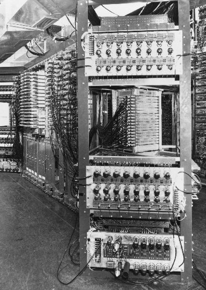
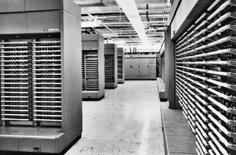
IBM received its first production contract in February 1954. The first AN/FSQ-7 was declared operational at McGuire Air Force Base, New Jersey, on July 1, 1958. IBM eventually manufactured 24 AN/FSQ-7s and 3 AN/FSQ-8s. Each AN/FSQ-7 weighed 250 tons, had a 3,000-kilowatt power supply and required 49,000 vacuum tubes. To ensure continuous operation each computer was duplexed; it actually consisted of two machines. The percentage of time that both machines in a system were down for maintenance was 0.043 percent, or 3.77 hours averaged over a year.
Software Development
In addition to the computer hardware, a large part of the air defense project effort was devoted to software development. The software task developed quickly into the largest real-time control program ever coded, and all the coding had to be done in machine language since higher-order languages did not yet exist. Furthermore, the code had to be assembled, checked, and realistically tested on a one-of-a-kind computer that was a shared test bed for software development, hardware development, demonstrations for visiting officials, and training of the first crew of Air Force operators.
The art of computer programming was essentially invented for SAGE.
Computer software was in an embryonic state at the beginning of the SAGE effort. In fact, the art of computer programming was essentially invented for SAGE. Among the innovations was more efficient programming (both in terms of computer run time and memory utilization), which was achieved through the use of generalized subroutines and which allowed the elimination of a one-to-one correspondence between the functions being carried out and the computer code performing these functions. A new concept, the central service (or bookkeeping) subprogram, was introduced.
Documentation procedures provided a detailed record of system operations and demonstrated the importance of system documentation. Checkout was made immensely faster and easier with utility subprograms that helped locate program errors. These general-purpose subprograms served, in effect, as the first computer compiler. The size of the program — 25,000 instructions — was extraordinary for 1955; it was the first large, fully integrated digital computer program developed for any application. Whirlwind was equal to the task: between June and November 1955, the computer operated on a 24-hour, 7-day schedule with 97.8 percent reliability.
Because of the complexity of the software, Lincoln Laboratory became one of the first institutions to enforce rigid documentation procedures. The software creation process included flow charts, program listings, parameter and assembly test specifications, system and program operating manuals, and operational, program, and coding specifications. About one-quarter of the instructions supported operational air defense missions. The remainder of the code was used to help generate programs, to test systems, to document the process, and to support the managerial and analytic chores essential to good software.
These programs were large, and because MIT did not want further increases in the Lincoln Laboratory staff, the Rand Corporation was asked to assist in the programming task. Rand was eager to play a role in the SAGE effort and began work on the software in April 1955. By December, the section of Rand in charge of SAGE programming — the System Development Division — had a staff of 500. Within a year, the System Development Division had a staff of a 1,000 and was larger than the rest of Rand put together. The Division left its parent company in November 1956 and formed the nonprofit System Development Corporation, with a $20 million contract to continue the work started by Rand and with additional contracts for programming the SAGE computers. SAGE had spawned another company, and another industry.
Cape Cod SAGE Prototype
While the Digital Computer Division at Lincoln Laboratory wrestled with Whirlwind, the Aircraft Control and Warning Division concentrated its efforts on verifying the underlying concepts of air defense. A key recommendation in the Project Charles Final Report was that a small air defense system should be constructed and evaluated before work on a more extensive system began. The report proposed that the experimental network be established in eastern Massachusetts, that it include 10 to 15 radars, and that all radars be connected to Whirlwind. This methodology of system prototyping, first established during SAGE, became core to Lincoln Laboratory's approach to the development of new system concepts, and is still very much part of the Laboratory's culture today.
As soon as the air defense program began, Lincoln Laboratory started to set up an experimental system and named it, for its location, the Cape Cod System. It was functionally complete; all air defense functions could be demonstrated, tested, and modified. The Cape Cod System was a model air defense system, scaled down in size but realistically embodying all operational functions.
Cape Cod, which was chosen because of its convenience to the Laboratory, was a good test site. It covered an area large enough for realistic testing of air defense functions. In addition, its location was challenging — hilly and bounded on two sides by the ocean, with highly variable weather and a considerable amount of air traffic.
Every aspect of the Cape Cod System called for innovation. Not only did it require radar netting, but radar data filtering was also needed to remove clutter that was not canceled by the moving-target indicator (MTI). Phone-line noise also had to be held within acceptable limits.
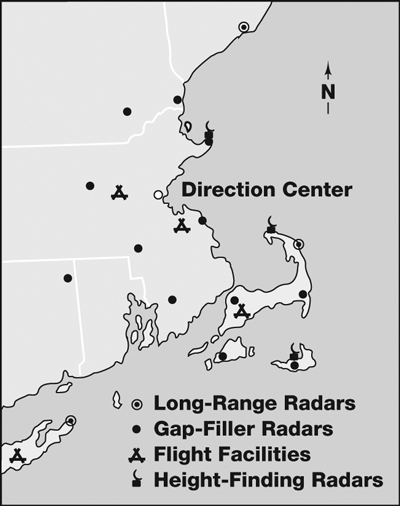
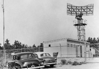
A long-range AN/FPS-3 radar, the workhorse of the operational air defense net, was installed at South Truro, Massachusetts, near the tip of Cape Cod, and equipped with an improved digital radar relay. Less powerful radars, known as gapfillers, were installed to enhance the coverage provided by the long-range system. Because near-total coverage was required, the beams of the radars in the network had to overlap, meaning that the radars could be separated by no more than 25 miles.

Initially, two SCR-584 radars that had been developed during World War II by the MIT Radiation Laboratory were installed as gapfillers at Scituate and Rockport, Massachusetts. Early tests of these radars showed much shorter detection ranges than expected, however, and improvements in the components and the test equipment were required to resolve the problems and make the radars operate as needed. As new radars became operational, each included a Mark-X identification-friend-or-foe (IFF) system, and reports were multiplexed with the radar data. Dedicated telephone circuits to the Barta Building in Cambridge were leased and tested.
Buffer storage had to be added to Whirlwind to handle the insertion of data from the asynchronous radar network, and the software had to be expanded considerably. A direction center needed to be designed and constructed to permit Air Force personnel to operate the system: to control the radar data filtering, initiate and monitor tracks, identify aircraft, and assign and monitor interceptors.
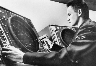
Construction of a realistic direction center depended heavily on the development of an interactive display console. Nothing comparable had ever been done before, and the technology was primitive. What was needed was a computer-generated display that would include alphanumeric characters (to act as labels on aircraft) and a separate electronic tote-board status display. Then, the console operator could select display categories of information (for example, hostile aircraft tracks) without being distracted by all of the information available.

The display console was developed around the Stromberg-Carlson Charactron cathode-ray tube (CRT). The tube contained an alphanumeric mask in the path of the electron beam. The beam was deflected to pass through the desired character on the mask, refocused, and then deflected a second time to the desired location on the tube face. This process was electronically complex, but it worked. The console operator had a keyboard for data input and a light-sensing gun, which was used to recognize positional information and enter it into the computer. This novel means of control for high-speed computers was invented at the Laboratory by Robert Everett.
All these complex engineering tasks were carried out in parallel, on schedule, and with little reworking. By September 1953, just two years and five months after the go-ahead, the Cape Cod System was fully operational. The radar network consisted of gapfiller radars, height-finding radars, and long-range radars.
The software program could handle, in abbreviated form, most of the air defense tasks of an operational system. Facilities were in place to initiate and track 48 aircraft, identify and find the height of targets, control 10 simultaneous interceptions from two air bases, and give early warning and transmit data on 12 tracks to an antiaircraft operations center. Now the system had to be tested.
Testing the Cape Cod System
Formal trials of the Cape Cod System began in October 1953, with flight tests two afternoons a week. The tests continued until June 15, 1954, and analysis of the initial test results was highly favorable. Track initiation, tracking, and identification were accomplished successfully.
Over the next few months, the Cape Cod System was expanded to include long-range AN/FPS-3 radars at Brunswick, Maine, and Montauk Point on the eastern tip of Long Island, New York. Additional gapfillers were built and integrated, completing the expanded radar network in the summer of 1954.
Jet interceptors were assigned to support the experiments: 12 Air Force F-89Cs at Hanscom Field and a group of Navy F-3Ds at South Weymouth, Massachusetts. Later, an operational Air Defense Command (ADC) squadron of F-86Ds based at the Suffolk County Airfield on Long Island was integrated into the Cape Cod System, and the Air Force arranged for Strategic Air Command training flights in the Cape Cod area so the Cape Cod System could be used for large-scale air defense exercises against Strategic Air Command B-47 jet bombers.

The time had come to test the Cape Cod System with a live interception. In a joint experiment with the MIT Instrumentation Laboratory (now the Charles Stark Draper Laboratory), a B-26 aircraft equipped with an autopilot was connected to the Whirlwind computer, and interceptor vectoring commands were transmitted automatically over the data link to the autopilot. The interception went as planned. The pilot soon sighted the target aircraft and let the autopilot complete a successful interception. Another important first had been accomplished.
The year 1955 was a watershed for the SAGE effort, with the focus of the program changing from installation and component testing to integrated system testing. The style of the program changed as well because the Air Force had given SAGE a precisely defined set of specifications.
On March 7, Air Defense Command (ADC) headquarters issued the Operational Plan for SAGE, prepared jointly by ADC and Lincoln Laboratory. The 300 pages provided "an overall understanding of the system, the concept of its operation, and the method by which it will be integrated into the Air Defense Command." The Operational Plan specified the equipment and personnel, the operational interactions between them, and their relationship within ADC. From that time on, work on SAGE had one overriding goal — to meet the specifications in the Operational Plan.
A new series of Cape Cod tests began in August 1955. Operator tasks in the direction center were changed so that they more closely resembled an actual SAGE subsector. Weapons-direction procedures were refined and training facilities were improved.
The basic concepts of automated air defense were demonstrated, and the tests showed that an automated air defense system could detect and intercept incoming aircraft.
The computer was able to process data from all 13 radars, and it could control manned interceptors and guide antiaircraft operation centers. The system had a capacity of 48 tracks that could be viewed in track situation displays, which geographically showed Air Defense Identification Zone lines and antiaircraft circles. Each console also had a 5-inch CRT for digital information display. Audible alert signals were used, with a different signal for each symbol on a situation display.
A major goal of the Cape Cod tests was to gather data that could be used for simulating interceptions. Simulations in the early series were based entirely on live tests, but the data gathered in 1955 made it possible to combine live clutter data and live flight data to create new combat situations. The ability to use test data to simulate new conditions was a ground-breaking innovation in computer programming. Outside Lincoln Laboratory, the simulations occasioned doubt and controversy, but the results of the simulations established their accuracy and realism, and they were ultimately accepted as a practical alternative and a valid part of test and training procedures.
Beginning in November 1955, Lincoln Laboratory initiated a set of system exercises with live aircraft, known as the System Operation Test (SOT) series. These tests were conducted in a series of missions of increasing complexity.
The Series I SOT comprised eight tests, flown between November 15, 1955, and January 31, 1956. During each test, B-29 strike aircraft made radial attacks against Boston, which was defended by aircraft from the Hanscom and South Weymouth air bases. A total of 50 aircraft were sent against the system. Against these aircraft, 62 interceptors were sent to defend the airspace, 24 of which successfully intercepted the strikes.
The Series II SOT, flown between February 14 and April 25, 1956, was still more dramatic and realistic. As many as 32 high-speed B-47 aircraft flown by the Strategic Air Command attacked targets in Boston as well as Martha's Vineyard, Massachusetts, and Portsmouth, New Hampshire. Raids included multiple aircraft performing complex maneuvers: flying less than 1,000 feet apart, making turns, and crossing, splitting, or joining tracks.
In the Series III SOT, carried out between July 6 and November 7, 1956, Boston was given a defense force of 16 interceptors from four air bases: Otis, Westover, Hanscom, and South Weymouth. Waves of B-47s attacked in groups of 12 to 16 aircraft, with the aircraft closely spaced and performing numerous crossing maneuvers.
The final series of Cape Cod System tests, carried out in 1957, focused on the development of new tracking techniques and new interception logic, and they produced significant results. The tests showed that, as long as the intercept-direction capacity was not exceeded, the Cape Cod System was capable of guiding interceptors sufficiently to achieve an interception rate of almost 100 percent.
The Cape Cod System was a great success for Lincoln Laboratory. The basic concepts of automated air defense were demonstrated, and the tests showed that an automated air defense system could detect and intercept incoming aircraft.
Success in the Cape Cod program, however, was not sufficient. The Operational Plan for SAGE called for a fully functional prototype, and the Cape Cod System was only a simplified model, with the most basic tracking and intercept-direction functions.
The Experimental SAGE Subsector

The Experimental SAGE Subsector (ESS) was essentially an expansion of the Cape Cod System. But, unlike the Cape Cod System, ESS was a fully operational prototype.
The emphasis during the ESS phase was on evaluation of the AN/FSQ-7(XD-1) computer before IBM began production of the AN/FSQ-7. ESS included most of the Cape Cod System sites, as well as some new ones, and it emulated the performance of an operational subsector. Radar data, aircraft flight plans, and meteorological information were transmitted automatically to the computer. The system was required to have overlapping radars, automatic crosstelling, height finding, a command post, and weather and weapons status totes. Radar coverage of the ESS represented a scaled SAGE subsector, although the boundaries actually overlapped the future McGuire, Stewart, and Brunswick subsectors.

The ESS direction center was located in Lincoln Laboratory's Building F, completed in 1955, and all ESS sites were connected to the AN/FSQ-7(XD-1). The computer occupied the first floor, the direction center was on the second floor, and the power equipment was in the basement.
The functionality needed for the direction center was defined as a set of specifications that were then coded as part of the direction center active (DCA) computer program. The DCA program was written in four successive packages, each of which performed a specific group of air defense functions. It eventually contained more than half a million lines of code and in excess of 25,000 instructions.

The conclusion of the Cape Cod System and Experimental SAGE Subsector prototyping activities signaled the end of an era for Lincoln Laboratory. The Laboratory had been founded as an institution for research and development, but the focus of its work was changing to operational testing and production. Both within Lincoln Laboratory and at MIT, concern was growing about the future of the program. Was it within Lincoln Laboratory's charter to produce an operational system? Or should Lincoln Laboratory, as a part of a great technical university, restrict its efforts to research and development? Within a year, these questions would break Lincoln Laboratory apart, and the Laboratory would transition SAGE to other organizations for implementation and move on to tackle other problems involving technology in the interest of national security.

Early-Warning Radars
Complementing the work on the Cape Cod System was an extensive radar development effort to increase response times through early-warning radars. Radar systems were developed for use in the air, over water, and in the Arctic. Although these radar developments were not formally part of the SAGE project, they were necessary to make the overall nation-wide air defense system work, and Lincoln Laboratory had a large role in their development.
In the summer of 1952, a group of scientists, engineers, and military personnel met at Lincoln Laboratory to consider ways to improve the air defense of North America. Headed by Jerrold Zacharias, the group included Albert Hill, director of Lincoln Laboratory, Herbert Weiss and Malcolm Hubbard, among others from the Laboratory, and a number of distinguished scientists, including J. Robert Oppenheimer, Isidor Rabi, and Robert Pound.
The 1952 Summer Study undertook the tasks of assessing the vulnerability of the United States to surprise air attack and of recommending ways to lessen that vulnerability. Since the greatest threat appeared to be an air attack by the Soviet Union via the North Pole, the study group focused its attention on the airspace above the 55th parallel, where Soviet bombers, having passed over the Pole, could fly undetected nearly to the border of the United States.
The plan for SAGE, already under way, was to detect, identify, track, and intercept just such aircraft. However, without early warning of an approaching attack, the readiness of interceptors and depth of airspace in which interception could take place would be drastically limited.
The Summer Study concluded it would be feasible to install a network of surveillance radars and communication links across northernmost North America from Alaska to Greenland that could give three to six hours' early warning against the threat envisioned. The results and recommendations of the study were briefed to key personnel of the Department of Defense (DoD) in late August 1952 and were well received.
The DEW Line
The DoD approved the 1952 Summer Study configuration for what would soon become known as the Distant Early Warning (DEW) Line and directed the Air Force to take immediate action to implement such a system. By December, the Air Force had awarded a contract to Western Electric for the construction and operation of a radar and communications network across northern Canada. The difficulties of installing, operating, and maintaining radars in the Arctic environment were immense, and the DEW Line, which became operational in 1957, remains an extraordinary feat of engineering.
Lincoln Laboratory provided numerous technical contributions to the DEW Line. One of the first issues the Summer Study had to resolve concerned the feasibility of long-distance communications in the Arctic. The frequent occurrence of solar disturbances in the far north ruled out the then standard forms of ionospheric-reflection HF communications. Fortunately, researchers at Lincoln Laboratory and MIT had already developed a better form of long-range communication — VHF ionospheric scatter propagation, which was not susceptible to solar disturbances.

VHF scatter propagation used the inhomogeneities of the ionosphere to provide a reliable method of long-distance communications, even in the Arctic. Solar disturbances did not disrupt this form of communications; in fact, they often improved it. Moreover, VHF scatter propagation required only moderate-power transmitters — 10 to 50 kilowatts. Until the advent of satellite communications, therefore, VHF scatter communications was able to provide a reliable method of rearward communications for the DEW Line. In addition, tropospheric scatter propagation, also investigated in large part by Lincoln Laboratory, was adopted for multichannel lateral communication between stations along the DEW Line.
Another issue discussed at meetings of the Summer Study was the staffing of the installations. It was clearly desirable to post as few technicians as possible at each site, and the automatic alerting radar developed by Lincoln Laboratory provided a way to reduce personnel requirements. An automatic alerting radar sounds an alarm whenever an aircraft enters the area of surveillance, thus freeing site technicians from 24-hour vigilance at the display scopes. This radar was especially useful in the far northern regions, because the display scopes were generally empty. With reasonably well-trained personnel, a typical site could be maintained with fewer than 20 technicians.
The X-1 automatic alerting radar was designed and fabricated in a five-month crash program at Lincoln Laboratory. Following the completion of this program, models X-2 through X-6 were designed and assembled in rapid succession for installation by Western Electric at test sites in Illinois and the Arctic. The design of the X-3 automatic alerting radar was turned over to Raytheon, and production models were installed along the DEW Line. This radar was designated the AN/FPS-19. This approach of prototyping first-of-a-kind articles, and then transitioning the design to industry for production, was established at Lincoln Laboratory during the SAGE era and is still in practice today.
Lincoln Laboratory also had a hand in developing a continuous-wave bistatic fence radar that was used as a gapfiller between AN/FPS-19 radars to detect low-flying aircraft. In the design of these radars, later designated AN/FPS-23, and in the improvement of large search radars, new techniques and components were introduced to decrease false-alarm rates and enhance automatic operation.
Lincoln Laboratory's efforts in radar design focused primarily on electrical engineering issues, but the high winds and extreme temperatures of the Arctic environment compelled Lincoln Laboratory to advance the mechanical engineering aspects of radars as well. Antenna shelters had to offer sufficient structural strength to withstand Arctic windstorms and still cause minimal attenuation of the radar beam. Before the development of the DEW Line, inflatable radomes had been occasionally used as antenna shelters, but inflatable radomes had great difficulty surviving Arctic conditions. Lincoln Laboratory solved this problem by developing rigid, electromagnetically transparent radomes. These radomes made possible not only uninterrupted operation of the DEW Line, but also a new generation of very large, precisely steerable antennas for long-range surveillance. This kind of rigid radome continues to be manufactured for many purposes.
Personnel in the newly formed Engineering Group approached Buckminster Fuller, inventor of the geodesic dome, and asked him for assistance in designing a rigid radome. Fuller suggested a three-quarter-sphere design and recommended polyester-bonded fiberglass, which offered a high strength-to-weight ratio, excellent weather resistance, and reasonable cost.

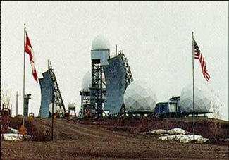
The concept of the geodesic dome seemed feasible, so the Engineering Group at Lincoln Laboratory procured a series of prototype rigid radomes. The first one (31-foot equatorial diameter) was erected on the roof of Building C. It was unexpectedly pummeled by Hurricane Carol in August 1954, with winds estimated up to 110 miles per hour, and no damage was inflicted. The radome was then disassembled and erected on Mount Washington in New Hampshire, and it successfully survived that mountain's fierce environment, where the highest wind speeds on the face of the earth have been recorded. A second 31-foot-diameter radome was erected over an AN/FPS-8 antenna on the roof of Building C. Tests demonstrated that the radome's effect on radar performance was negligible.

Lincoln Laboratory designed and procured a series of 50-foot-diameter rigid radomes that were installed in Thule, Greenland; Saglek Bay, Newfoundland; and Truro, Massachusetts. A second radome was also erected on the roof of Building C, where it sheltered the Sentinel antenna. The program culminated with the installation of a 150-foot-diameter radome at the Haystack Observatory.
Western Electric carried out the immense and highly successful project of installing the DEW Line radars. The DEW Line was completed in October 1962 with an extension to Iceland, giving the Air Force a 6,000-mile radar surveillance chain from the Aleutians to Iceland.
UHF Airborne Early-Warning Radars
Construction of the DEW Line resolved concerns about the security of the northern perimeter of the United States. But, as was recognized both during the 1952 Summer Study and subsequently, the DEW Line did nothing to reduce the vulnerability of the east and west coasts to an attack over the ocean.
With no land to the east or west of the United States, the logical counterpart to the DEW Line was airborne radar. The members of the Summer Study discussed the need for airborne early-warning (AEW) radar and identified the most important requirements.
In particular, they observed that it was more important to alert SAGE of distant aircraft intrusion than to control interceptors. Range resolution, azimuth resolution, and height-finding capability were, therefore, less important characteristics for AEW radars than sheer range. The need for the greatest possible range drove the use of a relatively low operating frequency because the transmitter powers available were greater at low frequency and the impact of clutter returns from the ocean on detection performance was less.
The Summer Study concluded that UHF AEW radar looked like a winner, and it proved to be just that. A program began at Lincoln Laboratory in the summer of 1952 to study existing radars and to test the feasibility of UHF radar. The first goal was to set up a UHF search radar to see if the hoped-for benefits were real. The frequency chosen for the first radar was 425 megahertz, primarily because a few dozen war-surplus Western Electric 7C22 dual-cavity triodes were available. Their limited mechanical tuning range covered that frequency. The experiments were successful and 425 megahertz became the frequency of choice for Lincoln Laboratory radars. In fact, Lincoln Laboratory's use of 425 megahertz for numerous subsequent radars followed directly from the availability of 7C22s in 1952.
In 1953, recognizing the importance of flight-test support for the development of AEW radars, the Navy established a unit at South Weymouth Naval Air Station, Massachusetts, to support several Lincoln Laboratory programs. The Air Force based an RC-121D and a B-29 at Hanscom Air Force Base for the same purpose.

An early demonstration of UHF AEW radar was on a Navy blimp. Its operating altitude was limited to a few thousand feet, but its comparatively low velocity made detection of airborne moving targets easier.
Flight testing commenced in March 1954. Side-by-side tests with a low-power UHF AEW radar in one blimp and an AN/APS-20 S-band AEW radar (developed by the Rad Lab during WWII) in another proved the advantage of lower-frequency operation.
Despite some advantages, blimps failed as AEW-radar platforms because their operation was restricted to low altitudes. However, heartened by successful flight tests in the blimp, Lincoln Laboratory set out to install an AEW radar in a Super Constellation-class aircraft and to increase the transmitted power.

The new radar, the AN/APS-70, was fielded in three experimental development versions. Two radars were built by Lincoln Laboratory, two by Hazeltine Electronics, and two by General Electric (GE). The broadband 425-megahertz antennas (including identification-friend-or-foe [IFF]) were supplied by Hughes. All three firms carried out production under contract to Lincoln Laboratory, and the technology was thus transferred to industry.
Lincoln Laboratory had demonstrated in 1954 that UHF AEW radar gave better results than S-band systems, but the Air Force felt that independent testing was warranted. Therefore, it carried out a series of flight-test comparisons of S-band and UHF AEW radars in 1956. In these tests, called Project Gray Wheel, an RC-121D aircraft was equipped with the AN/APS-20E (the most advanced configuration) S-band AEW radar, and another RC-121D aircraft was outfitted with Lincoln Laboratory's AN/APS-70 UHF AEW radar.
The tests proved the superiority of the UHF system in detecting bombers. Moreover, they demonstrated the capability of the UHF system to direct interceptors to the bombers. The success of the AN/APS-70-equipped aircraft helped convince the Air Force to outfit its fleet of RC-121 Super Constellations with UHF aircraft early-warning and control (AEW&C) radar.

Following the prototyping of the AN/APS-70, the Laboratory produced an improved UHF AEW radar prototype of the AN/APS-95 that featured single-knob tuning and other features not included in the AN/APS-70. Hazeltine produced the production AN/APS-95 UHF AEW radar for the Air Force, and GE produced an advanced version, the AN/APS-96 UHF AEW radar, for the Navy.
Even though UHF operation helped remove some sea clutter, a way to remove more of it without losing low-flying targets was badly needed. By 1952, long-range ground-based air-surveillance radars could discriminate between targets that were moving radially and those that were not by pulse-to-pulse subtraction of successive received signals after detection. However, the radar transmitter could not be counted on to produce the exact same frequency and starting phase each time it was pulsed, so the reference signal had to be coherently locked to the transmitted signal for every pulse.
Lincoln Laboratory developed a two-part solution to the detection of airborne targets in a clutter background, referred to as airborne moving-target indication (AMTI). First, the reference signal was locked to a sample of the clutter return from surface scatterers at close range. This technique was called time-averaged clutter-coherent airborne radar (TACCAR).
For moderate levels of sea clutter, TACCAR worked well. As the radar antenna scanned through 360 degrees in azimuth, TACCAR automatically took care of the problem of when the radar was looking forward or backward. The implementation of TACCAR at a radar's intermediate frequency (IF) was an early application of the phase-locked loop.
The second part of the solution was the displaced phase-center antenna (DPCA), first suggested by engineers at GE. DPCA compensated for the translation of an aircraft by comparing successive received pulses for AMTI and adjusting the phase center of the antenna to offset the phase difference between pulses caused by motion.
The Laboratory's existing UHF AEW-radar antennas were easily adapted to DPCA operation, and the integration of DPCA techniques with IF TACCAR was demonstrated by Lincoln Laboratory and was then implemented in the AN/APS-95.
Lincoln Laboratory subsequently demonstrated an RF version of TACCAR, which was made compatible with antijam circuitry. Because an airborne radar could be vulnerable to jamming, a tool kit was developed to strengthen the AN/APS-95 in this regard.
To improve target-detection performance and at the same time to narrow the beamwidth of the UHF radar, the Navy's Bureau of Aeronautics sponsored the installation of a large rotating radome high above the fuselage of a Super Constellation. One of Lincoln Laboratory's AN/APS-70 AEW radars was installed in the fuselage. Although the combination proved to be very effective, tests of the aircraft showed it was often on the verge of stalling.
By late 1957, the UHF AEW radars (with improved AMTI systems) had become accurate enough to be considered for incorporation into the SAGE system. To test the compatibility of the radars with SAGE, Lincoln Laboratory began the airborne long-range input (ALRI) test program.
The ALRI tests were conducted by flying an AN/APS-70–equipped AEW aircraft within line of sight of the Experimental SAGE Subsector installation at South Truro, Massachusetts. The video output from the radar's AMTI receiver was quantized and relayed to the ground over a wideband UHF data link. At the Experimental SAGE Subsector site, the data were fed into a fine-grain data system as if they were coming from a radar nearby. ALRI was a complex improvisation, but it worked.
The AMTI-radar technology that Lincoln Laboratory developed and demonstrated in the AN/APS-70 series of radars provided the foundation for the AN/APS-96. This radar used a high-power UHF vacuum-tube amplifier for the transmission of linear-FM pulse-compression signals. The finer-grained range resolution afforded by the compressed pulse after reception improved the target-to-sea-clutter ratio, making the AMTI job easier. The radar's sharper discrimination in range between closely spaced targets made the job of a combat information center easier. Another important feature was a height-finding capability for every target on every scan.
The Air Force retrofitted its RC-121C/Ds with Hazeltine AN/APS-95 UHF AEW radars, and the Navy installed General Electric AN/APS-96 UHF radars in Grumman W2F-1 Hawkeye turboprop aircraft.
Lincoln Laboratory's AEW radar program came to an end in the middle of 1959. Not only had the seven-year effort reopened the UHF spectrum for airborne radar applications, but highly effective AMTI systems had been developed and techniques needed to integrate AEW aircraft with SAGE had been demonstrated. Contractors were hard at work building radars that could apply these advances to Air Force and Navy aircraft. The Laboratory's assignment was complete.
The technologies developed as part of the Laboratory's AEW program continued to evolve and eventually became the bases of the Air Force's Airborne Warning and Control System (AWACS) and the Navy's E-2C airborne early-warning platforms. Parenthetically, years later the Laboratory re-engaged with the Air Force and Navy, and developed and prototyped key technologies for the next generations of these two systems. Airborne early warning is an active research area in the Laboratory today.
Jug Handle and Boston Hill Radars
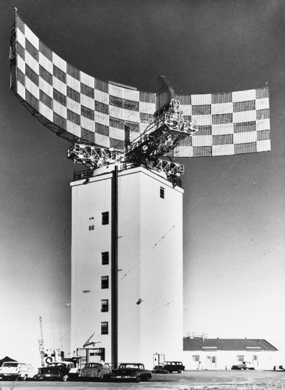
By 1954, it had become apparent that the L- and S-band ground control of intercept (GCI) radars used in the Cape Cod System were showing an unacceptable amount of clutter on their displays. At the same time, the ongoing development of UHF airborne early-warning (AEW) radar systems equipped with moving-target indication was demonstrating the advantages of radars operating at longer wavelengths. GCI radars operating at a longer wavelength appeared to address all of the problems that beset those at L- and S-band. However, the horizontal aperture of the rotating radar antenna would have to be larger in proportion to the wavelength in order to maintain the same angular resolution in azimuth. For the desired capabilities, the antenna had to be 120 feet wide by 16 feet high, but because its mechanical tolerances could be less stringent than those of an L-band antenna (because of its lower frequency), it was not expected to be a great challenge to construct.

The new UHF radar with the desired capabilities was designated the AN/FPS-31. A site was chosen on Jug Handle Hill in West Bath, Maine, which made the AN/FPS-31 the counterpart of shoreline GCI radars at South Truro, Massachusetts, and Montauk Point, New York.
The original design called for the rotating antenna to be carried on sets of bogie wheels at the ends of a three-armed spider that rolled on a smooth, level circular track at the top of the tower. This system caused trouble from the start. The track had not been made sufficiently smooth, and the wheels soon wore out. Pressure to get the AN/FPS-31 radar into operation led to the adoption of a scheme whereby the entire rotating assembly rode upon a large central ball. Although this modification presented its own challenges, the mechanical problems were eventually worked out and reliable operation of the large rotating antenna was achieved. The experience Lincoln Laboratory gained in solving these problems paid off in the subsequent successful mechanical designs of the counter-countermeasure (CCM) radar Mark I, the angle-tracking antenna of the Millstone radar, the AN/FPS-49 tracking radars, and others.
The AN/FPS-31 radar began to operate in October 1955. During the early checkout of the radar, echoes resembling returns from storms were observed. These turned out to be echoes from the aurora borealis — the Northern Lights. The radar was so sensitive that it could detect backscatter from the aurora high in the earth's atmosphere, far to the north.
In 1956, following assignment of the Jug Handle Hill radar to the SAGE Experimental Subsector, Lincoln Laboratory began work on an experimental advanced UHF radar to be used, in part, to evaluate new counter-countermeasure techniques. The experimental radar, designated as the CCM radar Mark I, was of particular importance because the UHF frequency range was to be employed in radar jammers then under development by the Soviet Union.
Design of the antenna and tower started in September 1956. In February 1957, an area on top of Boston Hill in North Andover, Massachusetts, was leased for the radar. Construction began immediately and the radar was first powered up in August 1958.
The main purpose of the Boston Hill radar was to serve as an instrumentation system for testing automatic detection and tracking of distant objects at a sufficiently high data rate to serve as an input to the SAGE system. The experimental work also emphasized measures designed to enable the radar to operate both actively and passively in a jamming environment.
Texas Towers
The final link in the early-warning network protecting the perimeter of the United States was a set of radar installations located in the Atlantic Ocean. In 1952, Lincoln Laboratory first suggested that permanent platforms be erected in shallow water at selected points along the Continental Shelf to provide a seaward extension of the radar warning system. These permanent marine radar stations were not inexpensive to build; nonetheless, they were both cheaper and more effective than radar picket ships, which were also employed at various times during the SAGE development.
|
The feasibility of long-distance communications was one of the main considerations in evaluating the practicality of a fixed marine radar station. Other radar stations used telephone lines and microwave line-of-sight radio for communications. The ocean-based towers, more than 100 miles offshore, could use neither. The conventional solution, transatlantic cable, was too expensive for the number of circuits needed. The solution to the long-range communications problem came from Lincoln Laboratory's development of UHF tropospheric scatter communication. In fact, the Texas Towers pioneered the use of UHF tropospheric scatter propagation for overwater communication. The UHF link between each tower and its direction center provided the equivalent of 72 four-wire telephone channels. Communication between each tower and aircraft for interceptor control was by line-of-sight UHF radio. Standing on 10-foot-diameter steel caissons driven into the sea floor, each Texas Tower was a half-acre steel island elevated 67 feet above the sea. The uppermost of the four decks carried three radomes, housing an AN/FPS-3 search radar and two AN/FPS-6 height-finding radars. The deck also held identification-friend-or-foe (IFF) equipment, a Mark X beacon, and four AN/FST-2 digital data transmitters. The remaining three decks housed the personnel and maintenance equipment, control equipment, water, and fuel. Fifty Air Force personnel, two meteorologists, and twenty civilians operated each station. The Air Force had approved five sites, but only Texas Towers 2, 3, and 4 were actually built. On January 15, 1961, Texas Tower 4 was destroyed by a winter storm. Tragically, none of the 28 airmen and civilian contractors who were manning the station survived. |

The sites of the Texas Tower radars are shown. Map courtesy of the Air Defense Online Radar Museum, www.radomes.org/museum

Photo of Texas Tower 2 on Georges Shoal, Massachusetts.

Photo of Tower 2, courtesy of the Air Defense Online Radar Museum.
|
Adapted from E.C. Freeman, ed., "Technology in the National Interest," Lexington, Mass.: MIT Lincoln Laboratory, 1995.
SAGE Transition
By the late 1950s, Lincoln Laboratory was becoming overwhelmed by the magnitude of its responsibilities for standing up the nation's first air defense system. The next phase of SAGE would be integrating interceptor weapons into the software, and that job was so massive that the Laboratory would have had to double in size. MIT, however, was unwilling to let Lincoln Laboratory grow any larger. Furthermore, the original purpose of the Laboratory — research and development — had nothing to do with system implementation of such a vast engineering task. Nonetheless, the SAGE program was continuing. Direction centers were under construction and weapons had begun to be integrated.
Late in 1957, Secretary of the Air Force James Douglas began a discussion with MIT about the future of the program. The Institute had grown increasingly reluctant to continue its involvement in a program that had less and less to do with research and more to do with implementation.
By 1957, Lincoln Laboratory had fulfilled its original charter. The Laboratory moved on to find new mission areas, particularly in ballistic missile defense and communications, and began to take on a new set of problems involving technology in the interest of national security.
The Air Force had approached multiple contractors, but they were either uninterested or unsuitable. What the Air Force needed was a contractor that understood the increasingly complex SAGE system, and Lincoln Laboratory was the only candidate.
Only one option was left — to create a new organization. The Secretary of the Air Force suggested that part of Lincoln Laboratory, the Digital Computer Division, be spun off from the rest of the Laboratory to continue the systems engineering for SAGE on its own. MIT agreed with the proposal, and the MITRE Corporation was established.
MITRE was incorporated as a nonprofit organization in July 1958, and Robert Everett left Lincoln Laboratory to become a technical director at MITRE. On January 1, 1959, 485 Lincoln Laboratory employees transferred to MITRE. Neither MIT nor Lincoln Laboratory would remain officially connected with MITRE, but the technical competence of the SAGE project was assured.
Lincoln Laboratory had fulfilled its original charter. With the departure of almost 500 personnel, the Laboratory became a much smaller organization. But after a pause for reevaluation, Lincoln Laboratory found new mission areas, particularly in the areas of ballistic missile defense and communications, and began to take on new problems involving technology in the interest of national security.
Reflections on SAGE
The SAGE period was unique in the history of Lincoln Laboratory and the nation. Only a few other programs — the Radiation Laboratory and the Manhattan Project being two prominent examples — had given scientists and engineers such a focused and rewarding experience.